Tutorial 2: Slide-seqV2, Slide-tags, or Stereo-seq

This tutorial guides through analysis of sequencing-based spatial transcriptomics data such as Slide-seqV2, Slide-tags, or Stereo-seq or any other similar technology. This tutorial do not require scRNA-seq reference data for integration, and assumes that cells were already annotated by another method (e.g. RCTD).

# if you installed the nico package

from nico import Annotations as sann
from nico import Interactions as sint
from nico import Covariations as scov

import matplotlib as plt

# if you did not install the nico package and downloaded the nico files into the current directory
#import Annotations as sann
#import Interactions as sint
#import Covariations as scov

#import scanpy as sc
#import gseapy
#import xlsxwriter

#import numpy as np
#import time
#import os

#import matplotlib as plt

plt.rcParams['pdf.fonttype'] = 42
plt.rcParams['ps.fonttype'] = 42
plt.rcParams['axes.linewidth'] = 0.1 #set the value globally

# please use Helvetica font according to your OS to ensure compatibility with Adobe Illustrator.
#plt.rcParams['font.family'] = 'Helvetica'
#plt.rcParams['font.sans-serif'] = ['Helvetica']

# Use the default font for all the figures
plt.rcParams['font.family'] = 'sans-serif'
plt.rcParams['font.sans-serif'] = ['Tahoma', 'DejaVu Sans','Lucida Grande', 'Verdana']

import warnings
warnings.filterwarnings("ignore")

print(nico.__version__)

1.4.0

Usage introduction

For details of the function usage and input parameters either refer to the documentation or just write the function and add .__doc__ to retrieve infromation on all relelvant parameters.

print(sann.find_anchor_cells_between_ref_and_query.__doc__) print(sint.spatial_neighborhood_analysis.__doc__) print(scov.gene_covariation_analysis.__doc__)

All the figures will be saved in saveas=pdf format as vector graphics by default. For every function that generates figures, the following default parameters are used: transparent_mode=False, saveas=‘pdf’,showit=True, dpi=300.

For saving figures in png format, set saveas=‘png’ For generating images without background, set transparent_mode=True. If figure outputs within the Jupyter Notebook are not desired, set showit=False.

Please download the sample data from the dropbox link and place the data in the following path to complete the tutorial: nico_cerebellum/cerebellum.h5ad

NiCoLRdb.txt (Ligand-receptor database file)

annotation_save_fname= ‘cerebellum.h5ad’ is the low resolution sequencing-based spatial transcriptomics file. In this anndata object, the adata.X contains the normalize count data,

adata.obsm[‘spatial’] for spatial coordinates,

adata.obsm[‘X_umap’] for 2D umap coordinates,

adata.obs[‘rctd_first_type’] contains the slot for cell type annotations,

and in the adata.raw.X slot contains the raw count matrix.

# parameters for saving plots

saveas='png'
transparent_mode=False

output_nico_dir='./nico_cerebellum/'
output_annotation_dir=output_nico_dir+'annotations/'
sann.create_directory(output_annotation_dir)

annotation_save_fname= 'cerebellum.h5ad'
#In this anndata .X slot contains the normalize matrix
# and in the .raw.X slot contains the count matrix

# parameters of the nico
inputRadius=0
annotation_slot='rctd_first_type' #spatial cell type slot

A: Visualize cell type annotation of spatial data

sann.visualize_umap_and_cell_coordinates_with_all_celltypes(
output_nico_dir=output_nico_dir,
output_annotation_dir=output_annotation_dir,
anndata_object_name=annotation_save_fname,
spatial_cluster_tag=annotation_slot,
spatial_coordinate_tag='spatial',
umap_tag='X_umap',
saveas=saveas,transparent_mode=transparent_mode)

The figures are saved:  ./nico_cerebellum/annotations/tissue_and_umap_with_all_celltype_annotations.png

Visualize spatial annotations of selected pairs (or larger sets) of cell types

Left side: tissue map, Right side: UMAP

choose_celltypes=[['Purkinje','Bergmann']]

# For visualizing every cell type individually, leave list choose_celltypes empty.
sann.visualize_umap_and_cell_coordinates_with_selected_celltypes(
output_nico_dir=output_nico_dir,
output_annotation_dir=output_annotation_dir,
anndata_object_name=annotation_save_fname,
spatial_cluster_tag=annotation_slot,
spatial_coordinate_tag='spatial',
umap_tag='X_umap',
choose_celltypes=choose_celltypes,
saveas=saveas,transparent_mode=transparent_mode)

The figures are saved:  ./nico_cerebellum/annotations/fig_individual_annotation/Purkinje0.png

B: Infer significant niche cell type interactions

Radius definition

If the radius in NiCo is set to R=0, NiCo incorporates the neighboring cells that are in immediate contact with the central cell to construct the expected neighborhood composition matrix. We envision NiCo as a method to explore direct interactions with physical neighbors (R=0), but in principle finite distance interactions mediated by diffusive factors could be explored by increasing R and comparing to the interactions obtained with R=0.

It may be helpful to explore a larger radius if it is expected that cell types interact through long-range interactions. However, during the covariation task, immediate neighbors typically capture the strongest signal, while a larger radius averages the signal from a bigger number of cells, potentially diluting the signal. Therefore, we recommend running NiCo with R=0.

Perform neighborhood analysis across direct neighbors (juxtacrine signaling, R=0) of the central niche cell type by setting inputRadius=0.

To exclude cell types from the neighborhood analysis, add celltype names to the list removed_CTs_before_finding_CT_CT_interactions. In the example below, the cell types nan, would not be included.

do_not_use_following_CT_in_niche=['nan']

niche_pred_output=sint.spatial_neighborhood_analysis(
Radius=inputRadius,
output_nico_dir=output_nico_dir,
anndata_object_name=annotation_save_fname,
spatial_cluster_tag=annotation_slot,
removed_CTs_before_finding_CT_CT_interactions=do_not_use_following_CT_in_niche)

average neighbors: 5.8214227309893705
average distance: 30.979645956596595
data shape (30569, 21) (30569,) neighbor shape (30569, 19)
Searching hyperparameters  Grid method: 0.000244140625
Searching hyperparameters  Grid method: 0.000244140625
Inverse of lambda regularization found 0.000244140625
training (24456, 19) testing (6113, 19) coeff (19, 19)

# this cutoff is use for the visualization of cell type interactions network
celltype_niche_interaction_cutoff=0.08

In some computing environments pygraphviz is not able to load the neato package automatically. In such cases, please define the location of the neato package. If you install pygraphviz through conda conda install -c conda-forge pygraphviz then most likely it should work.

import pygraphviz
a=pygraphviz.AGraph()
a._get_prog('neato')

import os
if  not '/home/[username]/miniforge3/envs/SC/bin/' in os.environ["PATH"]:
    os.environ["PATH"] += os.pathsep + '/home/[username]/miniforge3/envs/SC/bin/'

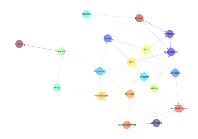
# Plot the niche interaction network with edge weight details for cutoff 0.08
sint.plot_niche_interactions_with_edge_weight(niche_pred_output,niche_cutoff=celltype_niche_interaction_cutoff,saveas=saveas,transparent_mode=transparent_mode)

The figures are saved:  ./nico_cerebellum/niche_prediction_linear/Niche_interactions_with_edge_weights_R0.png

# Plot the niche interaction network without any edge weight details for cutoff 0.08

sint.plot_niche_interactions_without_edge_weight(niche_pred_output,niche_cutoff=celltype_niche_interaction_cutoff,saveas=saveas,transparent_mode=transparent_mode)

The figures are saved:  ./nico_cerebellum/niche_prediction_linear/Niche_interactions_without_edge_weights_R0.png

Individual cell type niche plot

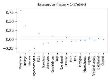
To plot regression coefficients of niche cell types for given central cell types, ordered by magnitude, add cell type names for the desired central cell types to the list argument choose_celltypes (e.g. Purkinje and Bergmann cells).

# Blue dotted line in following plot is celltype_niche_interaction_cutoff

sint.find_interacting_cell_types(niche_pred_output,choose_celltypes=['Purkinje','Bergmann'],
celltype_niche_interaction_cutoff=celltype_niche_interaction_cutoff,
saveas=saveas,transparent_mode=transparent_mode,figsize=(4.0,2.0))

The figures are saved:  ./nico_cerebellum/niche_prediction_linear/TopCoeff_R0/Rank2_Purkinje.png
The figures are saved:  ./nico_cerebellum/niche_prediction_linear/TopCoeff_R0/Rank6_Bergmann.png

If niche cell types from the niche neighborhood of all central cell types should be plotted or saved, then leave the choose_celltypes list argument empty.

#sint.find_interacting_cell_types(niche_pred_output,choose_celltypes=[])

# Plot the ROC curve of the classifier prediction for one of the cross-folds.
# sint.plot_roc_results(niche_pred_output,saveas=saveas,transparent_mode=transparent_mode)

Plot the average confusion matrix of the classifier from cross-folds:

sint.plot_confusion_matrix(niche_pred_output,
saveas=saveas,transparent_mode=transparent_mode)

The figures are saved:  ./nico_cerebellum/niche_prediction_linear/Confusing_matrix_R0.png

Plot the average coefficient matrix of the classifier from cross-folds:

sint.plot_coefficient_matrix(niche_pred_output,
saveas=saveas,transparent_mode=transparent_mode)

The figures are saved:  ./nico_cerebellum/niche_prediction_linear/weight_matrix_R0.png

#st.plot_predicted_probabilities(niche_pred_output)

Plot the evaluation score of the classifier for different metrics:

sint.plot_evaluation_scores(niche_pred_output,
saveas=saveas, transparent_mode=transparent_mode, figsize=(4,3))

The figures are saved:  ./nico_cerebellum/niche_prediction_linear/scores_0.png

C: Perform niche cell state covariation analysis using latent factors

Note: From module C onwards, Jupyter cells are independent of previous steps. Therefore, if you want to try different settings, you do not need to run the previous Jupyter cells.

Covariation parameter settings

Infer desired number of latent factors (e.g., no_of_factors=3) for each cell type. Here, we consider only the spatial modality and thus use conventional non-negative matrix factorization.

Set spatial_integration_modality=‘single’ for applying the conventional non-negative matrix factorization method on unimodal spatial data without integration.

In this case, latent factors will be derived from the spatial data alone.

Ligand-Receptor database file

NiCoLRdb.txt is the name of the ligand-receptor database file. Users can use databases of similar format from any resource.

NiCoLRdb.txt was created by merging ligand-receptor pairs from NATMI, OMNIPATH, and CellPhoneDB. It can be downloaded from github and saved in the local directory from where this notebook is run.

# By default, the function is run with spatial_integration_modality='double', i.e.
# it integrates spatial transcriptomics with scRNAseq data
# For running it only on spatial transcriptomics data, specify
# spatial_integration_modality='single'

cov_out=scov.gene_covariation_analysis(Radius=inputRadius,
no_of_factors=3,
spatial_integration_modality='single',
anndata_object_name=annotation_save_fname,
output_niche_prediction_dir=output_nico_dir,
ref_cluster_tag=annotation_slot) #LRdbFilename='NiCoLRdb.txt'

common genes between sc and sp 5160 5160


 Spatial and scRNA-seq number of clusters, respectively  19 19
Common cell types between spatial and scRNA-seq data   19 {'Lugaro', 'Ependymal', 'Candelabrum', 'Bergmann', 'Purkinje', 'Golgi', 'Fibroblast', 'Macrophages', 'MLI2', 'MLI1', 'Oligodendrocytes', 'Polydendrocytes', 'Endothelial', 'Granule', 'Microglia', 'Choroid', 'Globular', 'Astrocytes', 'UBCs'}

The spatial cluster name does not match the scRNA-seq cluster name  set()
If the above answer is Null, then everything is okay. However, if any spatial cell type does not exist in the scRNA-seq data, please correct this manually; otherwise, NiCo will not run.



Astrocytes alpha, H size, W size, spH size: 0 (3, 897) (4676, 3) (3, 897)
Bergmann alpha, H size, W size, spH size: 0 (3, 1534) (4802, 3) (3, 1534)
Candelabrum alpha, H size, W size, spH size: 0 (3, 42) (2823, 3) (3, 42)
Choroid alpha, H size, W size, spH size: 0 (3, 33) (2079, 3) (3, 33)
Endothelial alpha, H size, W size, spH size: 0 (3, 96) (2965, 3) (3, 96)
Ependymal alpha, H size, W size, spH size: 0 (3, 54) (2767, 3) (3, 54)
Fibroblast alpha, H size, W size, spH size: 0 (3, 307) (4206, 3) (3, 307)
Globular alpha, H size, W size, spH size: 0 (3, 15) (2104, 3) (3, 15)
Golgi alpha, H size, W size, spH size: 0 (3, 221) (4224, 3) (3, 221)
Granule alpha, H size, W size, spH size: 0 (3, 20575) (5147, 3) (3, 20575)
Lugaro alpha, H size, W size, spH size: 0 (3, 78) (3715, 3) (3, 78)
MLI1 alpha, H size, W size, spH size: 0 (3, 888) (4478, 3) (3, 888)
MLI2 alpha, H size, W size, spH size: 0 (3, 888) (4378, 3) (3, 888)
Macrophages alpha, H size, W size, spH size: 0 (3, 10) (642, 3) (3, 10)
Microglia alpha, H size, W size, spH size: 0 (3, 69) (2540, 3) (3, 69)
Oligodendrocytes alpha, H size, W size, spH size: 0 (3, 2087) (4797, 3) (3, 2087)
Polydendrocytes alpha, H size, W size, spH size: 0 (3, 113) (3538, 3) (3, 113)
Purkinje alpha, H size, W size, spH size: 0 (3, 2583) (4931, 3) (3, 2583)
UBCs alpha, H size, W size, spH size: 0 (3, 85) (3415, 3) (3, 85)

Visualize the cosine similarity and Spearman correlation between genes and latent factors

The following function generates output for the top 30 genes based on cosine similarity (left) or Spearman correlation (right) with latent factors.

Select cell types by adding IDs to the list argument choose_celltypes, or leave empty for generating output for all cell types.

scov.plot_cosine_and_spearman_correlation_to_factors(cov_out,
choose_celltypes=['Bergmann'],
NOG_Fa=30,
saveas=saveas,transparent_mode=transparent_mode,
figsize=(15,10))

cell types found  ['Bergmann']
The figures are saved:  ./nico_cerebellum/covariations_R0_F3/NMF_output/Bergmann.png

Visualizes genes associated with the latent factors along with average expression

Call the following function (scov.extract_and_plot_top_genes_from_chosen_factor_in_celltype) to visualize correlation and expression of genes associated with factors

For example, visualize and extract the top 20 genes (top_NOG=20) correlating negatively (positively_correlated=False) by Spearman correlation (correlation_with_spearman=True) for cell type Purkinje (choose_celltype=‘Purkinje’) to factor 1 (choose_factor_id=1)

dataFrame=scov.extract_and_plot_top_genes_from_chosen_factor_in_celltype(cov_out,
choose_celltype='Purkinje',
choose_factor_id=1,
top_NOG=20,correlation_with_spearman=True,positively_correlated=True,
saveas=saveas,transparent_mode=transparent_mode )

The figures are saved:  ./nico_cerebellum/covariations_R0_F3/dotplots/Factors_Purkinje.png

Inspect genes associated with a latent factor

Inspect the top genes associated with a the given factor. The table summarizes the positive or negative spearman correlation or cosine similarity with the factor, the mean expression and the proportion of cells expressing the gene for the respective cell type.

dataFrame

	Gene	Fa	mean_expression	proportion_of_population_expressed
0	Calb1	0.758210	4.204801	0.844367
1	Pcp4	0.757111	6.616725	0.932249
2	Car8	0.756901	6.302749	0.934959
3	Atp1b1	0.752535	3.228417	0.773906
4	Nsg1	0.735999	3.327526	0.803329
5	Itm2b	0.735834	3.303136	0.802555
6	Calm2	0.702097	2.882307	0.795587
7	Atp2a2	0.681419	2.284940	0.708866
8	Dner	0.670894	2.528068	0.749129
9	Pvalb	0.661823	3.056523	0.839334
10	Ckb	0.633108	3.635308	0.862176
11	Calm1	0.627708	2.569880	0.794812
12	Itpr1	0.609601	4.615563	0.900503
13	Ndrg4	0.603611	1.571816	0.638405
14	Pcp2	0.599627	3.116144	0.874952
15	Ppp1r17	0.595415	1.731707	0.671700
16	Ywhah	0.592602	1.284940	0.593496
17	Stmn3	0.575030	1.546264	0.654278
18	Nptn	0.555403	1.041038	0.530004
19	Mdh1	0.552998	1.429733	0.627178

Save the latent factors into an excel sheet

Save data in an excel sheet for each cell type, including latent factor associations of all genes according to Spearman correlation and cosine similarity.

scov.make_excel_sheet_for_gene_correlation(cov_out)

D: Cell type covariation visualization

Plot linear regression coefficients between factors of the central cell type (y-axis, defined by list argument choose_celltypes) and factors of niche cell types (x-axis).

Circle size scales with -log10(p-value) (indicated as number on top of each circle). To generate plots for all cell types, leave list argument choose_celltypes empty.

scov.plot_significant_regression_covariations_as_circleplot(cov_out,
choose_celltypes=['Bergmann'],
pvalue_cutoff=0.05,mention_pvalue=True,
saveas=saveas,transparent_mode=transparent_mode,
figsize=(6,1.25))

# In the following example, a p-value cutoff is explicitely defined by the pvalue_cutoff argument.
# p-value is printed as the -log10(p-value) on top of circle.
# circle color is the regression coefficients

cell types found  ['Bergmann']
The regression figures as pvalue circle plots are saved in following path  ./nico_cerebellum/covariations_R0_F3/Regression_outputs/pvalue_coeff_circleplot_*

Visualize as heatmap instead of circle plot

Plot regression coefficients between niche cell types (x-axis) and central cell type (y-axis, defined by list argument choose_celltypes) as heatmap.

Leave list argument choose_celltypes empty to generate plots for all cell types. The top subfigure shows the coefficients and bottom subfigure shows the -log10 p-values.

scov.plot_significant_regression_covariations_as_heatmap(cov_out,
choose_celltypes=['Bergmann'],
saveas=saveas,transparent_mode=transparent_mode, figsize=(6,1.25))

cell types found  ['Bergmann']
The regression figures as pvalue heatmap plots are saved in following path  ./nico_cerebellum/covariations_R0_F3/Regression_outputs/pvalue_coeff_heatmap_*

E: Analysis of ligand-receptor interactions between covarying niche cell types

Save excel sheets and summary in text file

Save all ligand-receptor interactions infered for the niche of each cell type in an excel sheet, and a summary of significant niche interactions in a text file.

scov.save_LR_interactions_in_excelsheet_and_regression_summary_in_textfile_for_interacting_cell_types(cov_out,
pvalueCutoff=0.05,correlation_with_spearman=True,
LR_plot_NMF_Fa_thres=0.1,LR_plot_Exp_thres=0.1,number_of_top_genes_to_print=5)

The Excel sheet is saved:  ./nico_cerebellum/covariations_R0_F3/Lig_and_Rec_enrichment_in_interacting_celltypes.xlsx
The text file is saved: ./nico_cerebellum/covariations_R0_F3/Regression_summary.txt

Usage for ligand-receptor visualizations

Perform ligand-receptors analysis In this example, output is generated for the ligand-receptor pairs associated with the intercting factor 1 of Bergmann cells and factor 1 of Purkinje cells.

choose_interacting_celltype_pair=[‘Bergmann’,‘Purkinje’]

choose_factors_id=[1,1] entries correspond to cell types in choose_interacting_celltype_pair, i.e., first factor ID corresponds to Bergmann and second factor ID corresponds to Purkinje.

By default, the analysis is saved in 3 separate figures (bidirectional, CC to NC and NC to CC). CC: central cell NC: niche cell

Our analysis accounts for bidirectional cellular crosstalk interactions of ligands and receptors in cell types A and B. The ligand can be expressed on cell type A and signal to the receptor detected on cell type B, or vice versa.

By changing the cutoff for minimum factor correlation of ligand/receptor genes (LR_plot_NMF_Fa_thres=0.2) or the cutoff for the minimum fraction of cells expressing the ligand/receptor genes (LR_plot_Exp_thres=0.2) the stringency of the output filtering can be controled.

scov.find_LR_interactions_in_interacting_cell_types(cov_out,
choose_interacting_celltype_pair=['Bergmann','Purkinje'],
choose_factors_id=[1,1],
pvalueCutoff=0.05,
LR_plot_NMF_Fa_thres=0.15,
LR_plot_Exp_thres=0.15,
saveas=saveas,transparent_mode=transparent_mode,figsize=(12, 10))

LR figures for both ways are saved in following path  ./nico_cerebellum/covariations_R0_F3/Plot_ligand_receptor_in_niche/
LR figures for CC to NC are saved in following path  ./nico_cerebellum/covariations_R0_F3/Plot_ligand_receptor_in_niche_cc_vs_nc/
LR figures for NC to CC are saved in following path  ./nico_cerebellum/covariations_R0_F3/Plot_ligand_receptor_in_niche_nc_vs_cc/

0

Perform ligand-receptors analysis of the Bergmann cell niche including all significant interaction partners.

choose_interacting_celltype_pair=[‘Bergmann’] generates plots for all cell types interacting sigificantly with Bergmann cells.

choose_factors_id=[] if empty, generates plots for all significantly covarying factors

# scov.find_LR_interactions_in_interacting_cell_types(all_output_data,choose_interacting_celltype_pair=['Bergmann'],
#   choose_factors_id=[], LR_plot_NMF_Fa_thres=0.2,LR_plot_Exp_thres=0.2,saveas=saveas,transparent_mode=transparent_mode)

F: Perform functional enrichment analysis for genes associated with latent factors

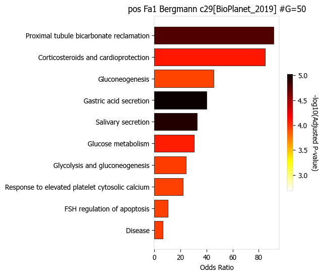
Perform pathway enrichment analysis for factor-associated genes

In this example, pathway analysis is performed for the top 50 (NOG_pathway=50) genes, positively correlated (positively_correlated=True) with factor 1 (choose_factors_id=[1]) of Bergmann cells (choose_celltypes=[‘Bergmann’]) testing for enrichment of Bioplanet 2019 (database=[‘BioPlanet_2019’]).

If savefigure=True, then the figures will be saved in the respective folder.

scov.pathway_analysis(cov_out,
choose_celltypes=['Bergmann'],
NOG_pathway=50,
choose_factors_id=[1],
positively_correlated=True,
display_plot_as='barplot',
object_for_color='Adjusted P-value',
object_for_xaxis='Odds Ratio',
savefigure=False,database=['BioPlanet_2019'])

The pathway figures are saved in  ./nico_cerebellum/covariations_R0_F3/Pathway_figures/
cell types found  ['Bergmann']

In this example, pathway analysis is performed for the top 50 (NOG_pathway=50) genes, postively correlated (positively_correlated=True) with factor 1 (choose_factors_id=[1]) of Purkinje cells (choose_celltypes=[‘Purkinje’]) testing for enrichment of GO Biological Processes (database=[‘BioPlanet_2019’]).

If savefigure=True, then the figures will be saved in the respective folder.

scov.pathway_analysis(cov_out,
choose_celltypes=['Purkinje'],
NOG_pathway=50,
choose_factors_id=[1],
positively_correlated=True,
display_plot_as='barplot',
object_for_color='Adjusted P-value',
object_for_xaxis='Odds Ratio',
savefigure=False,database=['BioPlanet_2019'])

The pathway figures are saved in  ./nico_cerebellum/covariations_R0_F3/Pathway_figures/
cell types found  ['Purkinje']

G: Visualization of top genes across cell types and factors as dotplot

Show the top 20 positively and negatively correlated genes (top_NOG=20) to the factors in visualize_factors_id and their average expression on a log scale for corresponding cell types indicated in choose_interacting_celltype_pair. In this example, plots are generated for factor 1 for Purkinje cells and factor 1 for Bergmann cells.

If the choose_celltypes=[], the plot will be generated for all cell types.

scov.plot_top_genes_for_pair_of_celltypes_from_two_chosen_factors(cov_out,
choose_interacting_celltype_pair=['Purkinje','Bergmann'],
visualize_factors_id=[1,1],
top_NOG=20,saveas=saveas,transparent_mode=transparent_mode)

The figures are saved:  ./nico_cerebellum/covariations_R0_F3/dotplots/combined_Purkinje_Bergmann.png

scov.plot_top_genes_for_a_given_celltype_from_all_factors(cov_out,
choose_celltypes=['Bergmann','Purkinje'],
top_NOG=20,saveas=saveas,transparent_mode=transparent_mode)

cell types found  ['Bergmann', 'Purkinje']
The figures are saved:  ./nico_cerebellum/covariations_R0_F3/dotplots/Bergmann.png
The figures are saved:  ./nico_cerebellum/covariations_R0_F3/dotplots/Purkinje.png

H: Visualize factor values in the UMAP

Visualize factor values for select cell types, e.g., Bergmann and Purkinje cells (choose_interacting_celltype_pair=[‘Bergmann’,’Purkinje’]) in scRNA-seq data umap. Select factors for each cell type (visualize_factors_id=[1,1]).

scov.visualize_factors_in_spatial_umap(cov_out,
visualize_factors_id=[1,1],
umap_tag='X_umap',
choose_interacting_celltype_pair=['Bergmann','Purkinje'],
saveas=saveas,transparent_mode=transparent_mode,figsize=(8,3.5))

The figures are saved:  ./nico_cerebellum/covariations_R0_F3/spatial_factors_in_umap.png

scov.visualize_factors_in_spatial_umap(cov_out,
visualize_factors_id=[1],
umap_tag='X_umap',
choose_interacting_celltype_pair=['Bergmann'],
saveas=saveas,transparent_mode=transparent_mode,figsize=(4,3.5))

The figures are saved:  ./nico_cerebellum/covariations_R0_F3/spatial_factors_in_umap.png