Tutorial 1: Single-Cell Resolution Spatial Transcriptomics (seqFISH, Xenium, or MERSCOPE etc.)
This tutorial demonstrates how to analyze single-cell resolution imaging-based spatial transcriptomics data such as generated by seqFISH, Xenium, and MERSCOPE. Please prepare the input files of scRNA-seq reference data and spatial transcriptomics data as described here.
# if you installed the nico package

from nico import Annotations as sann
from nico import Interactions as sint
from nico import Covariations as scov

import matplotlib as plt

# if you did not install the nico package and downloaded the nico files into the current directory
#import Annotations as sann
#import Interactions as sint
#import Covariations as scov

#import scanpy as sc
#import gseapy
#import xlsxwriter

#import numpy as np
#import time
#import os

#import matplotlib as plt
plt.rcParams['pdf.fonttype'] = 42
plt.rcParams['ps.fonttype'] = 42
plt.rcParams['axes.linewidth'] = 0.1 #set the value globally

# please use Helvetica font according to your OS to ensure compatibility with Adobe Illustrator.
plt.rcParams['font.family'] = 'Helvetica'
plt.rcParams['font.sans-serif'] = ['Helvetica']

# Use the default font for all the figures
plt.rcParams['font.family'] = 'sans-serif'
plt.rcParams['font.sans-serif'] = ['Tahoma', 'DejaVu Sans','Lucida Grande', 'Verdana']

import warnings
warnings.filterwarnings("ignore")
print(nico.__version__)
1.4.0
Usage introduction
For details of the function usage and input parameters either refer to
the documentation or just write the function and add .__doc__ to
retrieve information on all relelvant parameters.
print(sann.find_anchor_cells_between_ref_and_query.__doc__)
print(sint.spatial_neighborhood_analysis.__doc__)
print(scov.gene_covariation_analysis.__doc__)
All the figures will be saved in saveas=pdf format as vector
graphics by default. For every function that generates figures, the
following default parameters are used: transparent_mode=False,
saveas=‘pdf’,showit=True, dpi=300.
For saving figures in png format, set saveas=‘png’ For generating images without background, set transparent_mode=True. If figure output within the Jupyter Notebook is not desired, set showit=False.
Please download the sample data and python notebookds from the git repository and keep all the files and folders in the same directory to run the tutorial. Unzip inputRef.zip and inputQuery.zip.
inputRef (single-cell RNA-sequencing data)
inputQuery (single-cell resolution spatial transcriptomics data)
NiCoLRdb.txt (Ligand-receptor database file)
Before running the nico_analysis_highres_image_tech.ipynb notebook for the NiCo analysis, input data need to be prepared by running the Start_Data_prep.ipynb notebook. Once all the steps of Start_Data_prep.ipynb are completed, the following commands can be executed to run a complete NiCo aanlysis.
#parameters for saving plots
saveas='png'
transparent_mode=False
ref_datapath='./inputRef/'
query_datapath='./inputQuery/'


output_nico_dir='./nico_out/'
output_annotation_dir=None #uses default location
#output_annotation_dir=output_nico_dir+'annotations/'
annotation_save_fname= 'nico_celltype_annotation.h5ad'
inputRadius=0
The parameter denoting the cell type annotation slot for the scRNAseq data object is ref_cluster_tag.
For example, in an AnnData object the cell type annotation could be stored in adata.obs[‘cluster’].
ref_cluster_tag='cluster' #scRNAseq cell type slot
annotation_slot='nico_ct' #spatial cell type slot
A: Perform cell type annotation of the spatial data
The first step is finding anchor cells between two modalities:
anchors_and_neighbors_info=sann.find_anchor_cells_between_ref_and_query(
refpath=ref_datapath,
quepath=query_datapath,
output_nico_dir=output_nico_dir,
output_annotation_dir=output_annotation_dir)
Selection of parameters
NiCo’s cell type annotation relies on spatial Leiden cluster for guidance. These clusters can be inferred as demonstrated in the Start_Data_prep.ipynb notebook, e.g., with Leiden resolution parameter 0.4.
If you have a large number of cells (>200,000) and want to inspect cell type annotation using spatial Leiden clusters obtained with different Leiden resolution parameters (or any other parameter variations), save to the output_annotation_dir directory with a different name for each run.
MNN (Mutual Nearest Neighbors) alignment takes a considerable amount of time, which can slow down the analysis on an ordinary laptop. Therefore, it is advisable to save the anchors_data_50.npz file, as the anchor information is independent of the resolution parameter.
The annotation slot in the scRNA-seq data and initial cluster slot in the spatial data
ref_cluster_tag=‘cluster’ ### ref_cluster_tag defines the cell type slot in the scRNA-seq data. Example adata.obs[‘cluster’]. If the cell type annotation is stored in another slot please change the slot name.
guiding_spatial_cluster_resolution_tag=‘leiden0.4’ #### guiding_spatial_cluster_resolution_tag defines the Leiden cluster slot for spatial data. Example .obs[‘leiden0.4’]. If spatial guiding clusters are stored in another slot please change the slot name.
output_info=sann.nico_based_annotation(anchors_and_neighbors_info,
guiding_spatial_cluster_resolution_tag='leiden0.4',
across_spatial_clusters_dispersion_cutoff=0.15,
ref_cluster_tag=ref_cluster_tag,
resolved_tie_issue_with_weighted_nearest_neighbor='No')
The function sann.delete_files deletes the file with the anchor information
created by find_anchor_cells_between_ref_and_query. If you
have a large number of cells and want to experiment with different annotation
parameters, do not delete this file as it takes a significant amount
of time to compute.
sann.delete_files(output_info)
# Visualize the anchor cells between two modalities.
# sann.visualize_spatial_anchored_cell_mapped_to_scRNAseq(output_info)
Save the annotation file to an AnnData object
Save the annotation file to an AnnData object (annotation_save_fname) along with the spatial expression matrix in the “output_nico_dir” directory.
sann.save_annotations_in_spatial_object(output_info,
anndata_object_name=annotation_save_fname)
Nico cell type cluster are saved in following path './nico_out/' as <anndata>.obs['nico_ct'] slot
Note: Annotations from different computational methods such cell2location or TACCO
If you would like to use an available AnnData object with cell type annotations obtained with a different method, you can skip the previous steps.
To use your own annotations, replace the following file: annotation_save_fname= ‘nico_celltype_annotation.h5ad’ with annotation_save_fname= ‘other_method_celltype_annotations.h5ad’
The content of the AnnData object is as follows: The necessary slots are adata.obs[‘nico_ct’] or any other slot for cell type annotation, adata.obsm[‘spatial’] for spatial coordinates, adata.obsm[‘X_umap’] for 2D umap coordinates, adata.X is normalized count data, and adata.raw.X for raw count data.
>>> adata
    AnnData object with n_obs × n_vars = 7416 × 203
        obs: 'umi_sct', 'log_umi_sct', 'gene_sct', 'log_gene_sct', 'umi_per_gene_sct', 'log_umi_per_gene_sct', 'leiden0.4', 'leiden0.5', 'nico_ct'
        var: 'Intercept_sct', 'log_umi_sct', 'theta_sct', 'Intercept_step1_sct', 'log_umi_step1_sct', 'dispersion_step1_sct', 'genes_step1_sct', 'log10_gmean_sct'
        uns: 'leiden', 'leiden0.5_colors', 'neighbors', 'pca', 'umap'
        obsm: 'X_pca', 'X_umap', 'spatial'
        varm: 'PCs'
        obsp: 'connectivities', 'distances'
>>> adata.raw.X
    array([[ 0.,  0.,  0., ...,  0.,  0.,  9.],
           [ 0., 39.,  0., ...,  0.,  0.,  5.],
           [ 0., 49.,  0., ...,  0.,  0.,  4.],
           ...,
           [ 0.,  0.,  0., ...,  1.,  0.,  0.],
           [ 0.,  0.,  0., ...,  0.,  0.,  0.],
           [ 0.,  0.,  0., ...,  0.,  0.,  0.]], dtype=float32)
>>> adata.X.toarray()
    array([[ 0.        ,  0.        ,  0.        , ...,  0.        ,
                0.        ,  5.1008253 ],
           [ 0.        ,  8.992419  ,  0.        , ...,  0.        ,
                0.        ,  1.5530139 ],
           [ 0.        , 11.429277  ,  0.        , ...,  0.        ,
                0.        ,  1.1400297 ],
              ...,
           [ 0.        ,  0.        ,  0.        , ...,  0.47980395,
                0.        ,  0.        ],
           [ 0.        ,  0.        ,  0.        , ...,  0.        ,
                0.        ,  0.        ],
           [ 0.        ,  0.        ,  0.        , ...,  0.        ,
                0.        ,  0.        ]], dtype=float32)
Replace the AnnData object stored in annotation_save_fname with your own AnnData object containing the annotations. Ensure that the annotation slot name in your AnnData object is adjusted to ‘nico_ct’:
annotation_slot=‘nico_ct’
This will ensure compatibility with the NiCo pipeline.
Visualize the spatial annotations of all cell types
Left side: tissue map, Right side: UMAP
sann.visualize_umap_and_cell_coordinates_with_all_celltypes(
output_nico_dir=output_nico_dir,
output_annotation_dir=output_annotation_dir,
anndata_object_name=annotation_save_fname,
#spatial_cluster_tag='nico_ct',
spatial_cluster_tag=annotation_slot,
spatial_coordinate_tag='spatial',
umap_tag='X_umap',
saveas=saveas,transparent_mode=transparent_mode)
The figures are saved: ./nico_out/annotations/tissue_and_umap_with_all_celltype_annotations.png

Visualize spatial annotations of selected pairs (or larger sets) of cell types
Left side: tissue map, Right side: UMAP
choose_celltypes=[['Stem/TA','Paneth'],['Paneth','Goblet']]

sann.visualize_umap_and_cell_coordinates_with_selected_celltypes(
choose_celltypes=choose_celltypes,
output_nico_dir=output_nico_dir,
output_annotation_dir=output_annotation_dir,
anndata_object_name=annotation_save_fname,
spatial_cluster_tag=annotation_slot,spatial_coordinate_tag='spatial',umap_tag='X_umap',
saveas=saveas,transparent_mode=transparent_mode)
The figures are saved:  ./nico_out/annotations/fig_individual_annotation/Stem_TA0.png
The figures are saved:  ./nico_out/annotations/fig_individual_annotation/Paneth1.png


# For visualizing every cell type individually, leave list choose_celltypes list empty.
#sann.visualize_umap_and_cell_coordinates_with_selected_celltypes(choose_celltypes=[])
B: Infer significant niche cell type interactions
Radius definition
If the radius in NiCo is set to R=0, NiCo incorporates the neighboring cells that are in immediate contact with the central cell to construct the expected neighborhood composition matrix. We envision NiCo as a method to explore direct interactions with physical neighbors (R=0), but in principle finite distance interactions mediated by diffusive factors could be explored by increasing R and comparing to the interactions obtained with R=0.
It may be helpful to explore a larger radius if it is expected that cell types interact through long-range interactions. However, during the covariation task, immediate neighbors typically capture the strongest signal, while a larger radius averages the signal from a bigger number of cells, potentially diluting the signal. Therefore, we recommend running NiCo with R=0.
Perform neighborhood analysis across direct neighbors (juxtacrine signaling, R=0) of the central niche cell type by setting inputRadius=0.
To exclude cell types from the neighborhood analysis, add celltype names to the list removed_CTs_before_finding_CT_CT_interactions.
In the example below, the cell types Basophils, Cycling/GC B cell, and pDC, would not be included in the niche interaction task due to their low abundance.
do_not_use_following_CT_in_niche=['Basophils','Cycling/GC B cell','pDC']

niche_pred_output=sint.spatial_neighborhood_analysis(
Radius=inputRadius,
output_nico_dir=output_nico_dir,
anndata_object_name=annotation_save_fname,
spatial_cluster_tag='nico_ct',
removed_CTs_before_finding_CT_CT_interactions=do_not_use_following_CT_in_niche)
average neighbors: 4.83637851104445
average distance: 64.08306688807858
data shape (7305, 19) (7305,) neighbor shape (7305, 17)
Searching hyperparameters  Grid method: 0.015625
Searching hyperparameters  Grid method: 0.0078125
Searching hyperparameters  Grid method: 0.0078125
Inverse of lambda regularization found 0.0078125
training (5844, 17) testing (1461, 17) coeff (17, 17)
# this cutoff is used for the visualization of cell type interaction networks
celltype_niche_interaction_cutoff=0.1
In some computing environments pygraphviz is not able to load the neato
package automatically. In such cases, please define the location of the
neato package. If you install pygraphviz through conda
conda install -c conda-forge pygraphviz then most likely it should
work.
import pygraphviz
a=pygraphviz.AGraph()
a._get_prog('neato')

import os
if  not '/home/[username]/miniforge3/envs/SC/bin/' in os.environ["PATH"]:
    os.environ["PATH"] += os.pathsep + '/home/[username]/miniforge3/envs/SC/bin/'
Example A: Plot the niche interaction network without any edge weight details for cutoff 0.1
alpha parameter and change the colormap with input_colormap.
The popoular choice of colormaps are following: ‘summer’, ‘autumn’,
‘winter’, ‘cool’, ‘Wistia’, ‘hot’, ‘afmhot’, ‘gist_heat’,
‘copper’,‘Diverging’, ‘PiYG’, ‘PRGn’, ‘BrBG’, ‘PuOr’, ‘RdGy’, ‘RdBu’,
‘RdYlBu’, ‘RdYlGn’, ‘Spectral’, ‘coolwarm’, ‘bwr’, ‘seismic’, ‘flag’,
‘prism’, ‘ocean’, ‘gist_earth’, ‘terrain’,
‘gist_stern’,‘gist_rainbow’, ‘rainbow’, ‘jet’, ‘turbo’sint.plot_niche_interactions_without_edge_weight(niche_pred_output,
niche_cutoff=celltype_niche_interaction_cutoff,
saveas=saveas,
transparent_mode=transparent_mode,
showit=True,
figsize=(10,7),
dpi=dpi, #Resolution in dots per inch for saving the figure.
input_colormap='jet', #Colormap for node colors, from matplotlib colormaps.
with_labels=True, #Display cell type labels on the nodes, if True.
node_size=500, #Size of the nodes.
linewidths=0.5, #Width of the node border lines.
node_font_size=6, #Font size for node labels.
alpha=0.5, #Opacity level for nodes and edges. 1 is fully opaque, and 0 is fully transparent.
font_weight='bold' #Font weight for node labels; 'bold' for emphasis, 'normal' otherwise.
)
The figures are saved: ./nico_out/niche_prediction_linear/Niche_interactions_without_edge_weights_R0.png

Example B: Using edge weights included in the niche interaction plot can be done as shown below
sint.plot_niche_interactions_with_edge_weight(niche_pred_output,
niche_cutoff=celltype_niche_interaction_cutoff,
saveas=saveas,
transparent_mode=transparent_mode,
showit=True,
figsize=(10,7),
dpi=dpi,
input_colormap='jet',
with_labels=True,
node_size=500,
linewidths=1,
node_font_size=8,
alpha=0.5,
font_weight='normal',
edge_label_pos=0.35,   #Relative position of the weight label along the edge.
edge_font_size=3       #Font size for edge labels.
)
The figures are saved: ./nico_out/niche_prediction_linear/Niche_interactions_with_edge_weights_R0.png

Individual cell type niche plot
To plot regression coefficients of niche cell types for given central cell types, ordered by magnitude, add cell type names for the desired central cell types to the list argument choose_celltypes (e.g. Stem/TA and Paneth).
# Blue dotted line in the plot indicates celltype_niche_interaction_cutoff

sint.find_interacting_cell_types(niche_pred_output,
choose_celltypes=['Stem/TA','Paneth'],
celltype_niche_interaction_cutoff=celltype_niche_interaction_cutoff,
saveas=saveas,transparent_mode=transparent_mode,figsize=(4.0,2.0))
The figures are saved:  ./nico_out/niche_prediction_linear/TopCoeff_R0/Rank1_Paneth.png
The figures are saved:  ./nico_out/niche_prediction_linear/TopCoeff_R0/Rank3_Stem_TA.png


If regression coefficients for the niche neighborhoods of all cell types should be plotted or saved, then leave the choose_celltypes list argument empty.
#sint.find_interacting_cell_types(niche_pred_output,choose_celltypes=[])
# Plot the ROC curve of the classifier prediction for one of the crossfolds.
# sint.plot_roc_results(niche_pred_output,saveas=saveas,transparent_mode=transparent_mode))
# sint.plot_predicted_probabilities(niche_pred_output)
Plot the average confusion matrix of the classifier from cross-folds:
sint.plot_confusion_matrix(niche_pred_output,
saveas=saveas,transparent_mode=transparent_mode)
The figures are saved: ./nico_out/niche_prediction_linear/Confusing_matrix_R0.png

Plot the average coefficient matrix of the classifier from cross-folds:
sint.plot_coefficient_matrix(niche_pred_output,
saveas=saveas,transparent_mode=transparent_mode)
The figures are saved: ./nico_out/niche_prediction_linear/weight_matrix_R0.png

Plot the evaluation score of the classifier for different metrics:
sint.plot_evaluation_scores(niche_pred_output,
saveas=saveas, transparent_mode=transparent_mode,
figsize=(4,3))
The figures are saved: ./nico_out/niche_prediction_linear/scores_0.png

C: Perform niche cell state covariation analysis using latent factors
Note: From module C onwards, Jupyter cells are independent of the previous steps. Therefore, if you want to try different settings, you do not need to run the previous Jupyter cells.
Covariation parameter settings
Infer desired number of latent factors (e.g., no_of_factors=3) for each cell type from both modalities using integrated non-negative matrix factorization. Set iNMFmode=False for applying the conventional non-negative matrix factorization method. In this case, latent factors will be derived from the scRNA-seq data and transfered to the spatial modality.
This option is preferable if spatial data are affected by substantial technical noise due to unspecific background signal or gene expression spill-over between neighboring cell types due to imperfect segmentation.
Ligand-Receptor database file
NiCoLRdb.txt is the name of the ligand-receptor database file. Users can use databases of similar format from any resource.
NiCoLRdb.txt was created by merging ligand-receptor pairs from NATMI, OMNIPATH, and CellPhoneDB. It can be downloaded from github and saved in the local directory from where this notebook is run.
# By default, the function is run with spatial_integration_modality='double', i.e.
# it integrates spatial transcriptomics with scRNAseq data

cov_out=scov.gene_covariation_analysis(iNMFmode=True,
        Radius=inputRadius,
        no_of_factors=3,
        refpath=ref_datapath,
        quepath=query_datapath,
        spatial_integration_modality='double',
        output_niche_prediction_dir=output_nico_dir,
        ref_cluster_tag=ref_cluster_tag) #LRdbFilename='NiCoLRdb.txt'
common genes between sc and sp 203 203


 Spatial and scRNA-seq number of clusters, respectively  17 19
Common cell types between spatial and scRNA-seq data   17 {'cDC/monocyte', 'neurons/enteroendocrine', 'Lymphatic', 'Plasma', 'Stroma', 'Tuft', 'Macrophage', 'Goblet', 'Glial', 'Blood vasc.', 'Paneth', 'MZE', 'T cell', 'TZE', 'Rest B', 'BZE', 'Stem/TA'}

The spatial cluster name does not match the scRNA-seq cluster name  set()
If the above answer is Null, then everything is okay. However, if any spatial cell type does not exist in the scRNA-seq data, please correct this manually; otherwise, NiCo will not run.


BZE alpha, H size, W size, spH size: 30 (3, 325) (120, 3) (3, 1639)
Blood vasc. alpha, H size, W size, spH size: 28 (3, 33) (58, 3) (3, 148)
Glial alpha, H size, W size, spH size: 4 (3, 10) (44, 3) (3, 96)
Lymphatic alpha, H size, W size, spH size: 24 (3, 267) (97, 3) (3, 1301)
MZE alpha, H size, W size, spH size: 2 (3, 63) (60, 3) (3, 111)
Macrophage alpha, H size, W size, spH size: 16 (3, 89) (113, 3) (3, 346)
Paneth alpha, H size, W size, spH size: 12 (3, 128) (127, 3) (3, 184)
Plasma alpha, H size, W size, spH size: 16 (3, 85) (101, 3) (3, 439)
Rest B alpha, H size, W size, spH size: 12 (3, 234) (71, 3) (3, 48)
Stem/TA alpha, H size, W size, spH size: 8 (3, 420) (140, 3) (3, 1131)
Stroma alpha, H size, W size, spH size: 6 (3, 84) (107, 3) (3, 271)
T cell alpha, H size, W size, spH size: 46 (3, 54) (86, 3) (3, 488)
TZE alpha, H size, W size, spH size: 8 (3, 40) (72, 3) (3, 340)
Tuft alpha, H size, W size, spH size: 40 (3, 90) (68, 3) (3, 25)
cDC/monocyte alpha, H size, W size, spH size: 26 (3, 40) (86, 3) (3, 76)
neurons/enteroendocrine alpha, H size, W size, spH size: 2 (3, 26) (103, 3) (3, 250)
Visualize the cosine similarity and Spearman correlation between genes and latent factors
The following function generates output for the top 30 genes based on cosine similarity (left) or Spearman correlation (right) with latent factors.
Select cell types by adding IDs to the list argument choose_celltypes, or leave empty for generating output for all cell types.
scov.plot_cosine_and_spearman_correlation_to_factors(cov_out,
choose_celltypes=['Paneth'],
NOG_Fa=30,saveas=saveas,transparent_mode=transparent_mode,
figsize=(15,10))
cell types found  ['Paneth']
The figures are saved:  ./nico_out/covariations_R0_F3/NMF_output/Paneth.png

# Cosine and spearman correlation: visualize the correlation of genes from NMF
scov.plot_cosine_and_spearman_correlation_to_factors(cov_out,
choose_celltypes=['Stem/TA'],
NOG_Fa=30,saveas=saveas,transparent_mode=transparent_mode,
figsize=(15,10))
cell types found  ['Stem/TA']
The figures are saved:  ./nico_out/covariations_R0_F3/NMF_output/Stem_TA.png

Visualizes genes associated with the latent factors along with average expression
Call the following function (scov.extract_and_plot_top_genes_from_chosen_factor_in_celltype) to visualize correlation and expression of genes associated with factors.
For example, visualize and extract the top 20 genes (top_NOG=20) correlating negatively (positively_correlated=False) by Spearman correlation (correlation_with_spearman=True) for cell type Stem/TA (choose_celltype=‘Stem/TA’) to factor 1 (choose_factor_id=1)
dataFrame=scov.extract_and_plot_top_genes_from_chosen_factor_in_celltype(
cov_out,
choose_celltype='Stem/TA',
choose_factor_id=1,
top_NOG=20,
correlation_with_spearman=True,
positively_correlated=False,
saveas=saveas,transparent_mode=transparent_mode )
The figures are saved: ./nico_out/covariations_R0_F3/dotplots/Factors_Stem_TA.png

Inspect genes associated with a latent factor
Inspect the top genes associated with a the given factor. The table summarizes the positive or negative spearman correlation or cosine similarity with the factor, the mean expression and the proportion of cells expressing the gene for the respective cell type.
dataFrame
| Gene | Fa | mean_expression | proportion_of_population_expressed | |
|---|---|---|---|---|
| 0 | Chp2 | -0.626481 | 1.619048 | 0.388095 |
| 1 | Rbp7 | -0.623792 | 3.402381 | 0.504762 |
| 2 | Lgals3 | -0.584694 | 2.847619 | 0.480952 |
| 3 | St3gal4 | -0.575894 | 3.750000 | 0.492857 |
| 4 | Gm3336 | -0.563401 | 1.152381 | 0.383333 |
| 5 | Coro2a | -0.561060 | 2.904762 | 0.657143 |
| 6 | Dhrs11 | -0.558811 | 1.773810 | 0.585714 |
| 7 | Akr1c19 | -0.556204 | 1.142857 | 0.359524 |
| 8 | Cdkn2b | -0.555436 | 0.973810 | 0.257143 |
| 9 | Serpinb6a | -0.550037 | 7.459524 | 0.895238 |
| 10 | Slc51a | -0.549629 | 1.123810 | 0.333333 |
| 11 | Anxa2 | -0.545655 | 5.378572 | 0.761905 |
| 12 | Smim24 | -0.544530 | 11.040476 | 0.945238 |
| 13 | Apol10a | -0.541590 | 1.271429 | 0.297619 |
| 14 | Cyp4f40 | -0.535966 | 0.733333 | 0.326190 |
| 15 | Car4 | -0.535653 | 2.238095 | 0.464286 |
| 16 | Mall | -0.524968 | 0.778571 | 0.361905 |
| 17 | Anxa13 | -0.524648 | 2.526191 | 0.621429 |
| 18 | Pfkp | -0.520550 | 1.642857 | 0.483333 |
| 19 | 2200002D01Rik | -0.519799 | 8.476191 | 0.911905 |
Save the latent factors into an excel sheet
Save data in an excel sheet for each cell type, including latent factor associations of all genes according to Spearman correlation and cosine similarity.
scov.make_excel_sheet_for_gene_correlation(cov_out)
D: Cell type covariation visualization
Plot linear regression coefficients between factors of the central cell type (y-axis, defined by list argument choose_celltypes) and factors of niche cell types (x-axis).
Circle size scales with -log10(p-value) (indicated as number on top of each circle). To generate plots for all cell types, leave list argument choose_celltypes empty.
choose_celltypes=['Stem/TA']
scov.plot_significant_regression_covariations_as_circleplot(cov_out,
choose_celltypes=choose_celltypes,
mention_pvalue=True,
saveas=saveas,transparent_mode=transparent_mode,
figsize=(6,1.25))
cell types found  ['Stem/TA']
The regression figures as pvalue circle plots are saved in following path  ./nico_out/covariations_R0_F3/Regression_outputs/pvalue_coeff_circleplot_*

In the following example, a p-value cutoff is explicitely defined by the pvalue_cutoff argument and -log10(p-value) is not printed on top of the circles.
choose_celltypes=['Stem/TA']

scov.plot_significant_regression_covariations_as_circleplot(cov_out,
choose_celltypes=choose_celltypes,
pvalue_cutoff=0.05,mention_pvalue=False,
saveas=saveas,transparent_mode=transparent_mode,
figsize=(6,1.25))
cell types found  ['Stem/TA']
The regression figures as pvalue circle plots are saved in following path  ./nico_out/covariations_R0_F3/Regression_outputs/pvalue_coeff_circleplot_*

Visualize as heatmap instead of circle plot
Plot regression coefficients between niche cell types (x-axis) and central cell type (y-axis, defined by list argument choose_celltypes) as heatmap.
Leave list argument choose_celltypes empty to generate plots for all cell types. The top subfigure shows the coefficients and bottom subfigure shows the -log10 p-values.
scov.plot_significant_regression_covariations_as_heatmap(cov_out,
choose_celltypes=['Stem/TA'],
saveas=saveas,transparent_mode=transparent_mode, figsize=(6,1.25))
cell types found  ['Stem/TA']
The regression figures as pvalue heatmap plots are saved in following path  ./nico_out/covariations_R0_F3/Regression_outputs/pvalue_coeff_heatmap_*

E: Analysis of ligand-receptor interactions between covarying niche cell types
Save excel sheets and summary in text file
Save all ligand-receptor interactions infered for the niche of each cell type in an excel sheet, and a summary of significant niche interactions in a text file.
scov.save_LR_interactions_in_excelsheet_and_regression_summary_in_textfile_for_interacting_cell_types(cov_out,
pvalueCutoff=0.05,correlation_with_spearman=True,
LR_plot_NMF_Fa_thres=0.1,LR_plot_Exp_thres=0.1,number_of_top_genes_to_print=5)
The Excel sheet is saved:  ./nico_out/covariations_R0_F3/Lig_and_Rec_enrichment_in_interacting_celltypes.xlsx
The text file is saved: ./nico_out/covariations_R0_F3/Regression_summary.txt
Usage for ligand receptor visualizations
Perform ligand-receptors analysis. In this example, output is generated for the ligand-receptor pairs associated with the interacting factor 1 of Stem/TA cells and factor 1 of Paneth cells.
choose_interacting_celltype_pair=[‘Stem/TA’,‘Paneth’]
choose_factors_id=[1,1] entries correspond to cell types in choose_interacting_celltype_pair, i.e., first factor ID corresponds to Stem/TA and second factor ID corresponds to Paneth.
By default, the analysis is saved in 3 separate figures (bidirectional, CC to NC and NC to CC). CC: central cell NC: niche cell
Our analysis accounts for bidirectional cellular crosstalk interactions of ligands and receptors in cell types A and B. The ligand can be expressed on cell type A and signal to the receptor detected on cell type B, or vice versa.
By changing the cutoff for minimum factor correlation of ligand/receptor genes (LR_plot_NMF_Fa_thres=0.2) or the cutoff for the minimum fraction of cells expressing the ligand/receptor genes (LR_plot_Exp_thres=0.2) the stringency of the output filtering can be controled.
scov.find_LR_interactions_in_interacting_cell_types(cov_out,
choose_interacting_celltype_pair=['Stem/TA','Paneth'],
choose_factors_id=[1,1],
pvalueCutoff=0.05,
LR_plot_NMF_Fa_thres=0.3,
LR_plot_Exp_thres=0.2,
saveas=saveas,transparent_mode=transparent_mode,figsize=(12, 10))
LR figures for both ways are saved in following path  ./nico_out/covariations_R0_F3/Plot_ligand_receptor_in_niche/
LR figures for CC to NC are saved in following path  ./nico_out/covariations_R0_F3/Plot_ligand_receptor_in_niche_cc_vs_nc/
LR figures for NC to CC are saved in following path  ./nico_out/covariations_R0_F3/Plot_ligand_receptor_in_niche_nc_vs_cc/
0


Perform ligand-receptors analysis of the Paneth cell niche including all significant interaction partners.
choose_interacting_celltype_pair=[‘Paneth’] generates plots for all cell types interacting sigificantly with Paneth cells.
choose_factors_id=[] if empty, generate plots for all significantly covarying factors.
scov.find_LR_interactions_in_interacting_cell_types(cov_out,
choose_interacting_celltype_pair=['Paneth'],
choose_factors_id=[],
LR_plot_NMF_Fa_thres=0.2,
LR_plot_Exp_thres=0.2,
saveas=saveas,transparent_mode=transparent_mode,figsize=(12, 10))
LR figures for both ways are saved in following path  ./nico_out/covariations_R0_F3/Plot_ligand_receptor_in_niche/
LR figures for CC to NC are saved in following path  ./nico_out/covariations_R0_F3/Plot_ligand_receptor_in_niche_cc_vs_nc/
LR figures for NC to CC are saved in following path  ./nico_out/covariations_R0_F3/Plot_ligand_receptor_in_niche_nc_vs_cc/
0
F: Perform functional enrichment analysis for genes associated with latent factors
Example 1: Perform pathway enrichment analysis for factor-associated genes
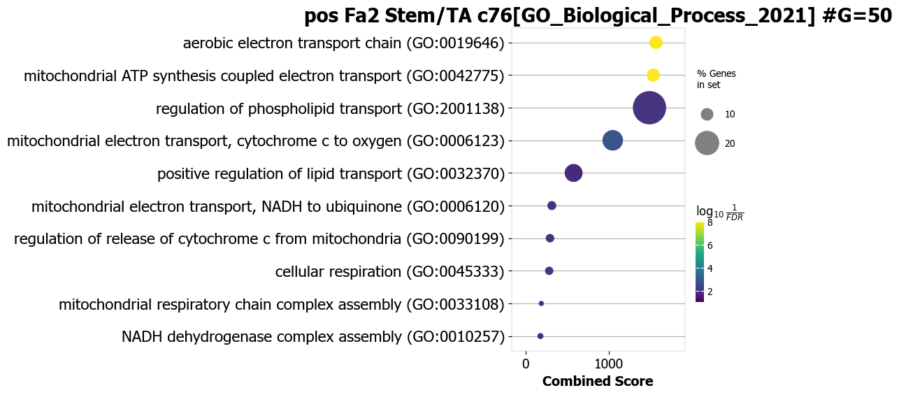
In this example, pathway analysis is performed for the top 50 (NOG_pathway=50) genes, positively correlated (positively_correlated=True) with factor 2 (choose_factors_id=[2]) of Stem/TA cells (choose_celltypes=[‘Stem/TA’]) testing for enrichment of GO Biological Processes (database=[‘GO_Biological_Process_2021’]).
If savefigure=True, then the figures will be saved in the respective folder.
scov.pathway_analysis(cov_out,
choose_celltypes=['Stem/TA'],
NOG_pathway=50,
choose_factors_id=[2],
savefigure=False,
positively_correlated=True,
saveas='pdf',
rps_rpl_mt_genes_included=False,
display_plot_as='dotplot',
correlation_with_spearman=True,
circlesize=12,
database=['GO_Biological_Process_2021'], #database=['BioPlanet_2019'],
object_for_color='Adjusted P-value',
object_for_xaxis='Combined Score',
fontsize=12,
showit=True,
input_colormap='viridis')
The pathway figures are saved in  ./nico_out/covariations_R0_F3/Pathway_figures/
cell types found  ['Stem/TA']

Example 2: increase the size of dot
scov.pathway_analysis(cov_out,
choose_celltypes=['Stem/TA'],
NOG_pathway=50,
choose_factors_id=[2],
savefigure=False,
positively_correlated=True,
saveas='pdf',
rps_rpl_mt_genes_included=False,
display_plot_as='dotplot',
correlation_with_spearman=True,
circlesize=20,
database=['GO_Biological_Process_2021'],
object_for_color='Adjusted P-value',
object_for_xaxis='Combined Score',
fontsize=12,
showit=True,
input_colormap='viridis')
The pathway figures are saved in  ./nico_out/covariations_R0_F3/Pathway_figures/
cell types found  ['Stem/TA']
Example 3: instead of dotplot show as a barplot
scov.pathway_analysis(cov_out,
choose_celltypes=['Stem/TA'],
NOG_pathway=50,
choose_factors_id=[2],
positively_correlated=True,
database=['GO_Biological_Process_2021'], #database=['BioPlanet_2019'],
rps_rpl_mt_genes_included=False,
display_plot_as='barplot',
correlation_with_spearman=True,
object_for_color='Adjusted P-value',
object_for_xaxis='Combined Score',
showit=True,
input_colormap='hot_r')
The pathway figures are saved in  ./nico_out/covariations_R0_F3/Pathway_figures/
cell types found  ['Stem/TA']

Example 4 (Recommended version): We recommend using the following version of the plot
scov.pathway_analysis(cov_out,
choose_celltypes=['Stem/TA'],
NOG_pathway=50,
choose_factors_id=[2],
positively_correlated=True,
database=['GO_Biological_Process_2021'], #database=['BioPlanet_2019'],
rps_rpl_mt_genes_included=False,
display_plot_as='barplot',
correlation_with_spearman=True,
object_for_color='Adjusted P-value',
object_for_xaxis='Odds Ratio',
showit=True,
input_colormap='hot_r')
The pathway figures are saved in  ./nico_out/covariations_R0_F3/Pathway_figures/
cell types found  ['Stem/TA']

Example 5
In this example, pathway analysis is performed for the top 50 (NOG_pathway=50) genes, negatively correlated (positively_correlated=False) with factor 2 (choose_factors_id=[2]) of Stem/TA cells (choose_celltypes=[‘Stem/TA’]) testing for enrichment of GO Biological Processes (database=[‘GO_Biological_Process_2021’]).
scov.pathway_analysis(cov_out,
choose_celltypes=['Stem/TA'],
NOG_pathway=50,
choose_factors_id=[2],
positively_correlated=False,
database=['GO_Biological_Process_2021'], #database=['BioPlanet_2019'],
rps_rpl_mt_genes_included=False,
display_plot_as='barplot',
correlation_with_spearman=True,
object_for_color='Adjusted P-value',
object_for_xaxis='Odds Ratio',
showit=True,
input_colormap='hot_r')
The pathway figures are saved in  ./nico_out/covariations_R0_F3/Pathway_figures/
cell types found  ['Stem/TA']

Example 6
In this example, pathway analyses are performed for the top 50 (NOG_pathway=50) genes, positively correlated (positively_correlated=True) with any factor (choose_factors_id=[]) of Paneth cells (choose_celltypes=[‘Paneth’]), ribosome and mitochondrial genes are not included in the gene list testing for enrichment of pathways from three databases (GO_Biological_Process_2021, BioPlanet_2019, Reactome_2016).
scov.pathway_analysis(cov_out,
choose_celltypes=['Paneth'],
NOG_pathway=50,
choose_factors_id=[],
positively_correlated=True,
savefigure=False,
rps_rpl_mt_genes_included=False,
#database=['GO_Biological_Process_2021'], #database=['BioPlanet_2019'],
display_plot_as='barplot',
object_for_color='Adjusted P-value',
object_for_xaxis='Odds Ratio',
showit=True,
input_colormap='hot_r')
The pathway figures are saved in  ./nico_out/covariations_R0_F3/Pathway_figures/
cell types found  ['Paneth']


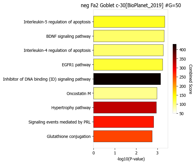
Example 7
In this example, pathway analysis is performed for negatively correlated (positively_correlated=False) with factor 2 (choose_factors_id=[2]) of Goblet cells (choose_celltypes=[‘Goblet’]) testing for enrichment of BioPlanet pathways (database=[‘BioPlanet_2019’]). Object_for_color=‘Odds Ratio’ and Object_for_xaxis=‘Adjusted P-value’
scov.pathway_analysis(cov_out,
choose_celltypes=['Goblet'],
NOG_pathway=50,
choose_factors_id=[2],
positively_correlated=False,
savefigure=False,
rps_rpl_mt_genes_included=False,
database=['BioPlanet_2019'],
display_plot_as='barplot',
object_for_color='Odds Ratio',#columntag  P-value,Adjusted P-value,Old P-value,Old Adjusted P-value,
object_for_xaxis= 'Adjusted P-value',#Odds Ratio', #'Combined Score'
showit=True,
input_colormap='hot_r')
The pathway figures are saved in  ./nico_out/covariations_R0_F3/Pathway_figures/
cell types found  ['Goblet']

Example 8
Object_for_color=‘Combined Score’ and Object_for_xaxis=‘P-value’
scov.pathway_analysis(cov_out,
choose_celltypes=['Goblet'],
NOG_pathway=50,
choose_factors_id=[2],
positively_correlated=False,
savefigure=False,
rps_rpl_mt_genes_included=False,
database=['BioPlanet_2019'],
display_plot_as='barplot',
object_for_color='Combined Score',#columntag  P-value,Adjusted P-value,Old P-value,Old Adjusted P-value,
object_for_xaxis= 'P-value',#Odds Ratio', #'Combined Score'
showit=True,
input_colormap='hot_r')
The pathway figures are saved in  ./nico_out/covariations_R0_F3/Pathway_figures/
cell types found  ['Goblet']
G: Visualization of top genes across cell types and factors as dotplot
Show the top 20 positively and negatively correlated genes (top_NOG=20) for all latent factors and the average expression of these genes on a log scale in a single plot. In this example, plots are generated for Paneth and Stem/TA cells.
If choose_celltypes=[], the plot will be generated for all cell types.
scov.plot_top_genes_for_a_given_celltype_from_all_factors(
cov_out,choose_celltypes=['Paneth','Stem/TA'],
top_NOG=20,saveas=saveas,transparent_mode=transparent_mode)
cell types found  ['Paneth', 'Stem/TA']
The figures are saved:  ./nico_out/covariations_R0_F3/dotplots/Paneth.png
The figures are saved:  ./nico_out/covariations_R0_F3/dotplots/Stem_TA.png


scov.plot_top_genes_for_pair_of_celltypes_from_two_chosen_factors(cov_out,
choose_interacting_celltype_pair=['Stem/TA','Paneth'],
visualize_factors_id=[1,1],
top_NOG=20,saveas=saveas,transparent_mode=transparent_mode)
The figures are saved: ./nico_out/covariations_R0_F3/dotplots/combined_Stem_TA_Paneth.png

H: Visualize factor values in the UMAP
Visualize factor values for select cell types, e.g., Stem/TA and Paneth cells (choose_interacting_celltype_pair=[‘Stem/TA’,‘Paneth’]) in scRNA-seq data umap. Select factors for each cell type (visualize_factors_id=[1,1]).
List entries correspond to cell types in choose_interacting_celltype_pair.
scov.visualize_factors_in_scRNAseq_umap(cov_out,
choose_interacting_celltype_pair=['Stem/TA','Paneth'],
visualize_factors_id=[1,1],
saveas=saveas,transparent_mode=transparent_mode,figsize=(8,3.5))
The figures are saved: ./nico_out/covariations_R0_F3/scRNAseq_factors_in_umap.png
0

Visualize factor values for select cell types, e.g., Stem/TA and Paneth cells (choose_interacting_celltype_pair=[‘Stem/TA’,’Paneth’]) in the spatial transcriptomics data UMAP. Select factors for each cell type (visualize_factors_id=[1,1]). List entries correspond to cell types in choose_interacting_celltype_pair.
scov.visualize_factors_in_spatial_umap(cov_out,
visualize_factors_id=[1,1],
choose_interacting_celltype_pair=['Stem/TA','Paneth'],
saveas=saveas,transparent_mode=transparent_mode,figsize=(8,3.5))
The figures are saved: ./nico_out/covariations_R0_F3/spatial_factors_in_umap.png
0

#For visualization of one cell type at a time only


scov.visualize_factors_in_spatial_umap(cov_out,
visualize_factors_id=[2],
choose_interacting_celltype_pair=['Stem/TA'],
saveas=saveas,transparent_mode=transparent_mode,figsize=(4,3.5))

scov.visualize_factors_in_scRNAseq_umap(cov_out,
#refpath=ref_datapath,
choose_interacting_celltype_pair=['Stem/TA'],
visualize_factors_id=[2],
saveas=saveas,transparent_mode=transparent_mode,figsize=(4,3.5))
The figures are saved:  ./nico_out/covariations_R0_F3/spatial_factors_in_umap.png
The figures are saved:  ./nico_out/covariations_R0_F3/scRNAseq_factors_in_umap.png
0

