Tutorial 0: Data Preparation
This tutorial guides through data preparation for tutorial 1. For the input data and the jupyter notebook file please use the following link
import scanpy as sc
import matplotlib.pyplot as plt
import numpy as np
import pandas as pd
import os
#import pickle
#from scipy.spatial import cKDTree
#from SCTransform import SCTransform

# if you installed the nico package
import nico
from nico import Annotations as sann

# if you did not install the nico package and downloaded the nico files into the current directory
# import Annotations as sann


import warnings
import time
warnings.filterwarnings('ignore')
#export PYTHONWARNINGS='ignore:Multiprocessing-backed parallel loops:UserWarning'
os.environ["PYTHONWARNINGS"] = "ignore::UserWarning"
Usage introduction
Please download the sample data from the git repository nico_tutorial and keep all the files and folders in the same directory to complete the tutorial. Unzip inputRef.zip and inputQuery.zip.
inputRef (single-cell RNA-sequencing data)
inputQuery (single-cell resolution spatial transcriptomics data)
NiCoLRdb.txt (Ligand-receptor database file)
The following notebook normalizes the count data and computes the initial Leiden clustering for the spatial transcriptomics data to perform the cell type annotation using NiCo: Start_Data_prep.ipynb
Once all the steps of the data preparation notebook are finalized, run the core notebook to perform the full NiCo analysis: nico_analysis_highres_image_tech.ipynb
print(nico.__version__)
1.4.0
# These are the input data paths for the scRNA-seq and spatial data
# If the data is not in h5ad or csv format then please adjust following the standard scanpy routine.

scdatapath='./inputRef/'
spdatapath='./inputQuery/'

ad_spatial_ori=sc.read(spdatapath+'gene_by_cell.csv').transpose()
ad_seq_ori=sc.read_h5ad(scdatapath+'input_ref.h5ad')

# This is the coordinate file of the cell centroids from the spatial transcriptomics experiment.
coordinate = pd.read_csv(spdatapath+'tissue_positions_list.csv')
coordinate=coordinate.to_numpy()
# make sure that the order of cells in the count matrix and in the cell location
# matrix are identical (command should return TRUE); otherwise correct the order

np.array_equal(coordinate[:,0],ad_spatial_ori.obs_names)
True
ad_spatial_ori.obsm['spatial']=coordinate[:,1:].astype(float)
If a spatial h5ad object is already available:
If spatial data in h5ad format with coordinate information tagged as spatial (.obsm[‘spatial’]) is already available, the previous commands can be skipped and the spatial data directly loaded:
ad_spatial_ori=sc.read_h5ad(spdatapath+‘input_query_spatial_data.h5ad’)
# data size of the variables
print(ad_spatial_ori)
print(ad_seq_ori)
print(coordinate.shape)
AnnData object with n_obs × n_vars = 7416 × 241
    obsm: 'spatial'
AnnData object with n_obs × n_vars = 2239 × 32287
    obs: 'cluster'
(7416, 4)
# Filter the cells and genes
sc.pp.filter_cells(ad_spatial_ori, min_counts=5)
sc.pp.filter_cells(ad_seq_ori, min_counts=5)

sc.pp.filter_genes(ad_spatial_ori, min_cells=1)
sc.pp.filter_genes(ad_seq_ori, min_cells=1)

print(ad_spatial_ori)
print(ad_seq_ori)
AnnData object with n_obs × n_vars = 7416 × 241
    obs: 'n_counts'
    var: 'n_cells'
    obsm: 'spatial'
AnnData object with n_obs × n_vars = 2239 × 21197
    obs: 'cluster', 'n_counts'
    var: 'n_cells'
Reference scRNA-seq data
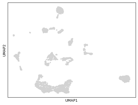
Copy the scRNA-seq data into a new variable as well as into the raw layer. The Original_count count matrix will be used to derive the UMAP for the scRNA-seq data. The raw layer count matrix will be used to find the Spearman and Cosine similarity of genes with the latent factors.
Original_counts=ad_seq_ori.copy()
Original_counts.raw=Original_counts.copy()
# Standard scanpy analysis

sc.pp.normalize_total(Original_counts)
sc.pp.log1p(Original_counts)

sc.tl.pca(Original_counts)
sc.pp.neighbors(Original_counts)
sc.tl.umap(Original_counts)
sc.pl.umap(Original_counts)
OMP: Info #276: omp_set_nested routine deprecated, please use omp_set_max_active_levels instead.
# save the data
Original_counts.write_h5ad(scdatapath+'Original_counts.h5ad')
Perform scTransform-normalization (Pearson residuals) with two different alternative stratgies
# Alternative 1
# The sctransform normalization function from scanpy

'''
ad_seq_common.raw=ad_seq_common.copy()
ad_spatial_common.raw=ad_spatial_common.copy()
# perform scTranform normalization common gene space for spatial data and scRNAseq data
sc.experimental.pp.normalize_pearson_residuals(ad_seq_common,inplace=True) #ad_seq_common.X[ad_seq_common.X<0]=0

ad_seq_common.write_h5ad(scdatapath+'sct_singleCell.h5ad')
sc.experimental.pp.normalize_pearson_residuals(ad_spatial_common,inplace=True) #ad_spatial_common.X[ad_spatial_common.X<0]=0
#print(ad_spatial_common.X.toarray()
'''
"nad_seq_common.raw=ad_seq_common.copy()nad_spatial_common.raw=ad_spatial_common.copy()n# perform scTranform normalization common gene space for spatial data and scRNAseq data nsc.experimental.pp.normalize_pearson_residuals(ad_seq_common,inplace=True) #ad_seq_common.X[ad_seq_common.X<0]=0nnad_seq_common.write_h5ad(scdatapath+'sct_singleCell.h5ad')nsc.experimental.pp.normalize_pearson_residuals(ad_spatial_common,inplace=True) #ad_spatial_common.X[ad_spatial_common.X<0]=0n#print(ad_spatial_common.X.toarray()n"
# Alternative 2
# The normalization using an external functions
# In the manuscript, this functions was used

temp_spatial=ad_spatial_common.copy()
temp_seq=ad_seq_common.copy()

sct_ad_sp = sann.SCTransform(ad_spatial_common,min_cells=1,gmean_eps=1,n_genes=500,n_cells=None, #use all cells
                        bin_size=500,bw_adjust=3,inplace=False)

sct_ad_sc = sann.SCTransform(ad_seq_common,min_cells=1,gmean_eps=1,n_genes=500,n_cells=None, #use all cells
                            bin_size=500,bw_adjust=3,inplace=False)

ad_spatial_common=sct_ad_sp.copy()
ad_seq_common=sct_ad_sc.copy()

ad_spatial_common.raw=temp_spatial.copy()
ad_seq_common.raw=temp_seq.copy()
ad_spatial_common.obsm['spatial']= temp_spatial.obsm['spatial']

ad_seq_common.write_h5ad(scdatapath+'sct_singleCell.h5ad')
Perform Leiden clustering on spatial transcriptomics data to guide cell type annotation
# standard scanpy analysis
sc.pp.pca(ad_spatial_common)
sc.pp.neighbors(ad_spatial_common,n_pcs=30)
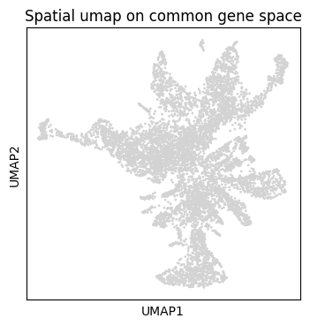
sc.tl.umap(ad_spatial_common)
# visualize umap
plt.rcParams["figure.figsize"] = (4, 4)
sc.pl.umap(ad_spatial_common, title=["Spatial umap on common gene space"],wspace=0.4,show=True)
Guiding Leiden cluster resolutions
Peform Leiden clustering for several resolution parameters. If it takes a long time to compute, then you can limit the number of parameters.
Any of the resolution parameters here can be used as an input parameter (guiding_spatial_cluster_resolution_tag) in the NiCo pipeline
#sc.tl.leiden(ad_spatial_common, resolution=0.3,key_added="leiden0.3")
sc.tl.leiden(ad_spatial_common, resolution=0.4,key_added="leiden0.4")
sc.tl.leiden(ad_spatial_common, resolution=0.5,key_added="leiden0.5")
#sc.tl.leiden(sct_ad_sp, resolution=0.6,key_added="leiden0.6")
#sc.tl.leiden(sct_ad_sp, resolution=0.7,key_added="leiden0.7")
#sc.tl.leiden(sct_ad_sp, resolution=0.8,key_added="leiden0.8")
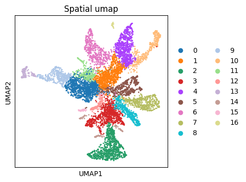
# Visualize your initial spatial clustering in the umap
# A good resolution parameter should yield clusters corresponding to major cell types.

sc.pl.umap(ad_spatial_common, color=["leiden0.5"], title=["Spatial umap"],wspace=0.4,
           show=True, save='_spatial_umap.png')
WARNING: saving figure to file figures/umap_spatial_umap.png
# Save the Leiden clusters for all resolution parameters as well as normalized count data in h5ad format.
ad_spatial_common.write_h5ad(spdatapath+'sct_spatial.h5ad')